Hachure In development
Status · in development

Hachure is not released and is not available to download. It is a working application under active development - everything on this page is produced by code in the repository, and everything described is built unless it says otherwise. Numbers, panels and behaviour will change.

Remote sensing analysis · macOS

Every band, every bit, at the speed you can look.

Hachure is a macOS workstation for quantitative remote sensing, built to be quick to reach for and quick to answer. Landsat 4 through 9, Sentinel-1 and 2, MODIS, VIIRS, ASTER, SPOT 1 through 7, Pléiades and Pléiades Neo, WorldView-2/3 and Legion, GeoEye-1, SkySat and the PlanetScope Doves are first-class citizens - their bands, wavelengths, ground sample distances and calibration equations are already known, so an index written once resolves on any of them. Aerial photography, LiDAR surfaces, hyperspectral cubes and towed conductivity surveys open in the same window.

Sensors known20 +
Public archives5
Native bit depth8 / 16 / 32
RequiresmacOS 26 · Apple silicon

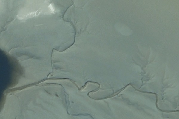
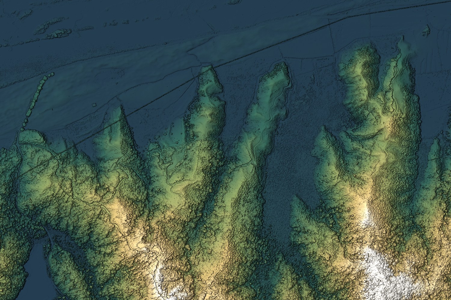
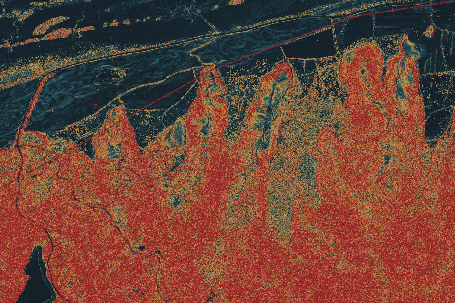
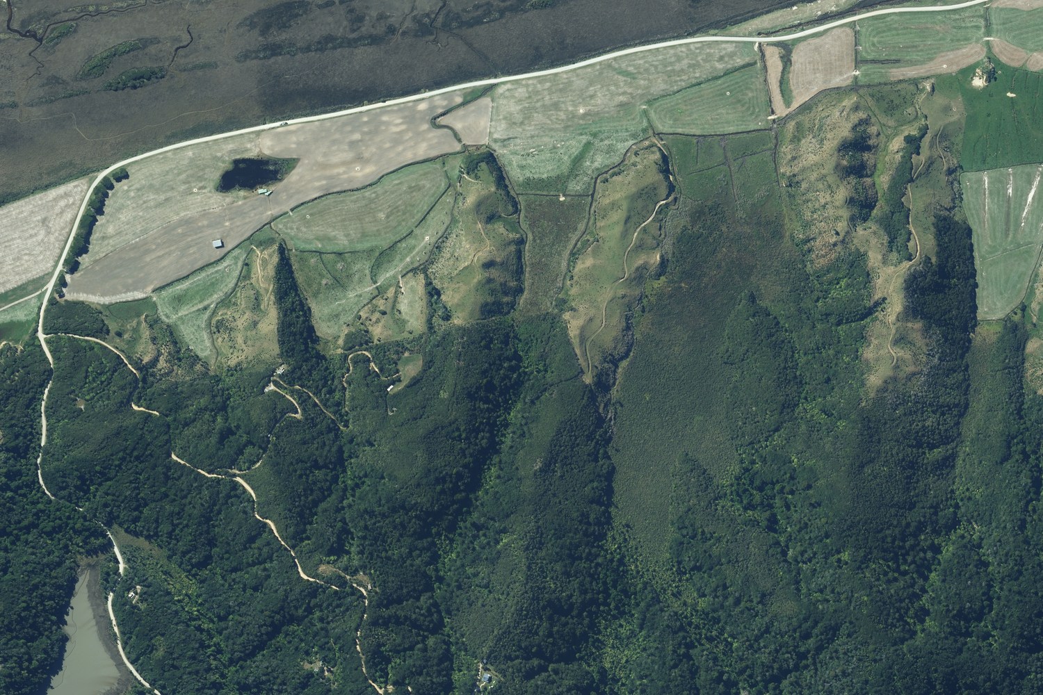
Plotted above: hachures traced down the gradient of a 1 m LiDAR surface, Whanganui Inlet, north-west Nelson. Stroke weight follows slope, after Lehmann (1799). The same ground appears photographically further down.

Finding dataWhere the time goes

Five public archives, searched in place

Most of the time spent on a scene is spent before it opens: working out which archive holds it, drawing the area again in someone's web viewer, downloading four candidates to find the one the cloud missed. Hachure searches five public archives from the window you are already working in - Earth Search on AWS, Microsoft Planetary Computer, CNES GEODES, the Alaska Satellite Facility and LINZ - and shows you enough to choose before anything is fetched.
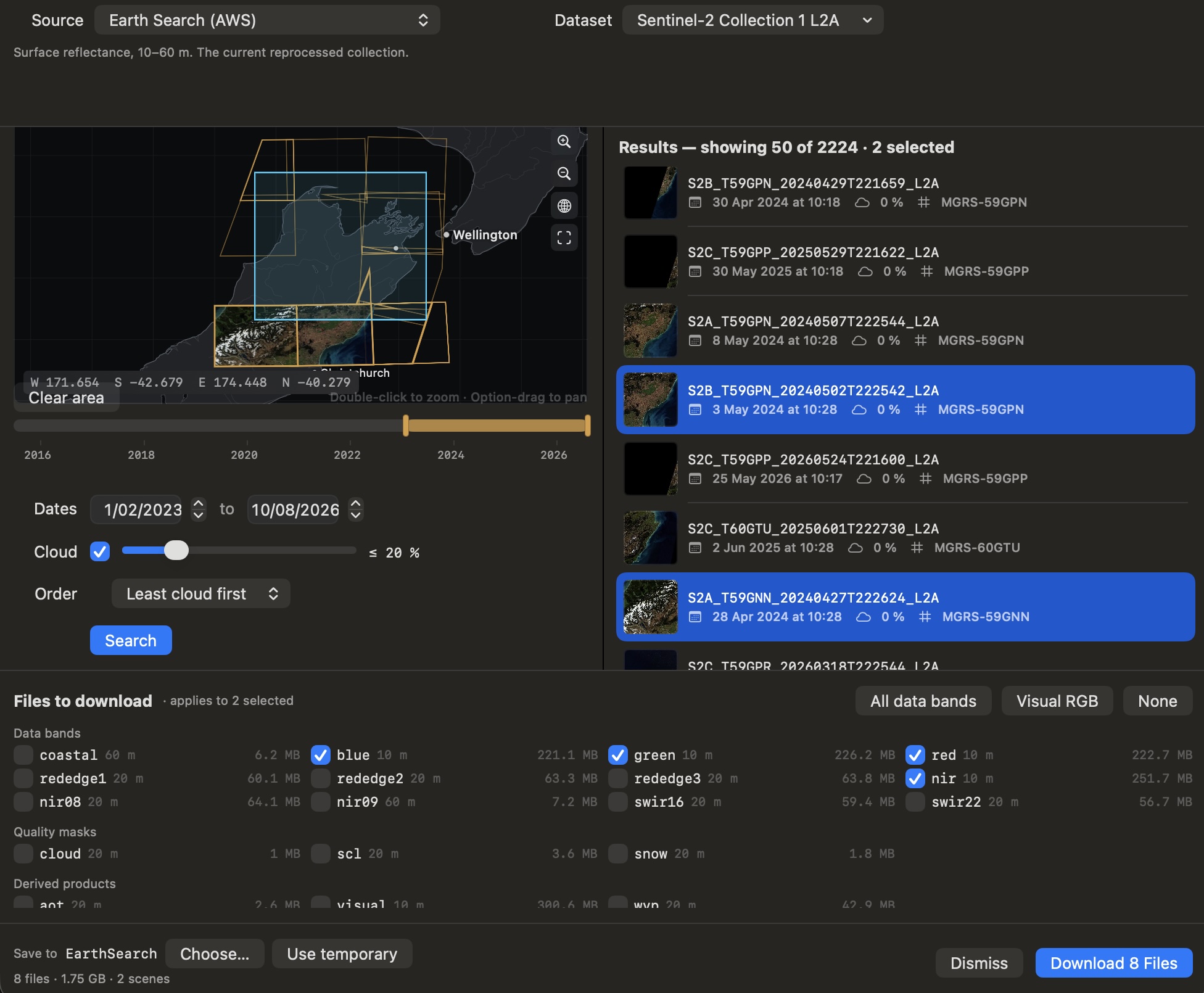
Import Scenes on Earth Search with the world map, timeline range bar and cloud filter
File ▸ Import from Earth Search ⇧⌘I Sentinel-2 L2A · cloud ≤ 20 % · least cloud first

Area of interest

If a raster is open, its extent is one click: the panel offers Extent of <that raster> and seeds the search area from it, correctly projected, with no coordinates typed and no box redrawn by eye. That is the common case - you have a scene and you want the one before it, or the same ground from a different sensor - and it is the one that usually costs the most fiddling elsewhere. Otherwise drag a box on the built-in world map, which works offline.

Date range and cloud filter

The date range is a draggable span drawn over the archive's own temporal extent, so a window that cannot contain anything is visibly one: SPOT 2's imagery begins in 1990, and a search from 1986 shows you the four years it is wasting rather than returning nothing and leaving you to guess why. Cloud cover is a slider where the collection reports it, and quietly absent where it does not, because a filter that silently does nothing is worse than no filter. Results sort by least cloud first.

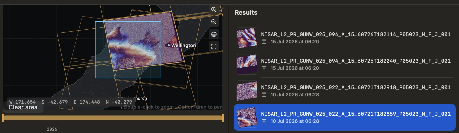
Search results with each scene's browse image drawn on the map inside its own footprint over the area of interest
Previews on the AOI NISAR L2 GUNW each quicklook inside its own footprint the selected scene under a brighter outline

Where an archive publishes a browse image, it is drawn on the map, inside the scene's own footprint, over your area of interest - so you can see at a glance whether the cloud is over the ground you care about or off in a corner. That is the question a percentage cannot answer: a scene at 18 % cloud is useless if all of it sits on your paddock. Thumbnails load only for rows that appear and are cached per scene, so scrolling a long result list does not fetch fifty images.

Placement is taken seriously rather than approximated. A browse image is positioned by its scene's bounding box, so any transparent margin inside the picture is ground it claims and does not have - on a real radar quicklook that was 27.5 % of the canvas above the swath, which drew the data a fifth of a box too far south. Trimming to the opaque content puts the four points where the swath meets its own envelope within 0.15 – 0.73 % of where the archive's geometry says they are. The trim is on alpha only, never brightness, because a dark margin and a dark coastline are the same pixels.

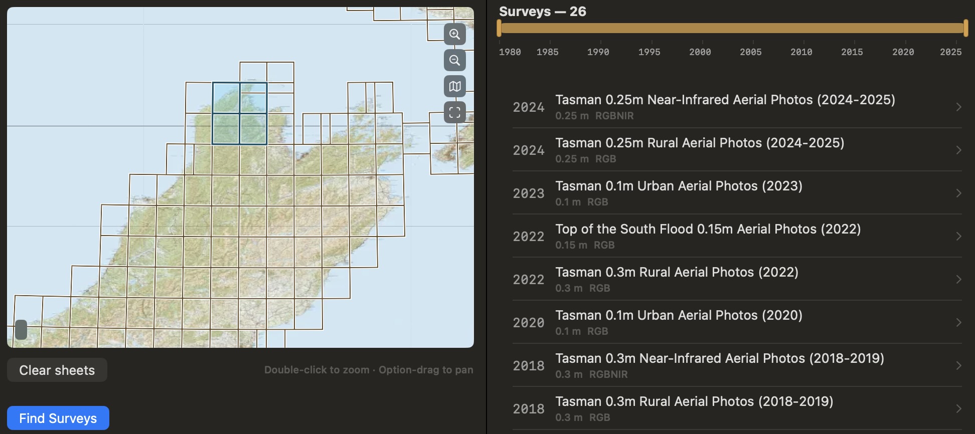
LINZ: selection by map sheet

LINZ publishes a static catalogue rather than a search service, so it is selected by Topo50 sheet. Click the sheets you want and Find Surveys asks the bucket which aerial surveys hold tiles for them - over a single sheet that answer is a time series of the same ground across decades, narrowed by the years they were flown. Nothing is fetched to find out: one listing request per survey answers whether it covers your ground at all.

Import Scenes on LINZ with the Topo50 sheet grid and a list of surveys
Sheets → surveys 80 surveys over two sheets newest first, narrowed by the years they were flown
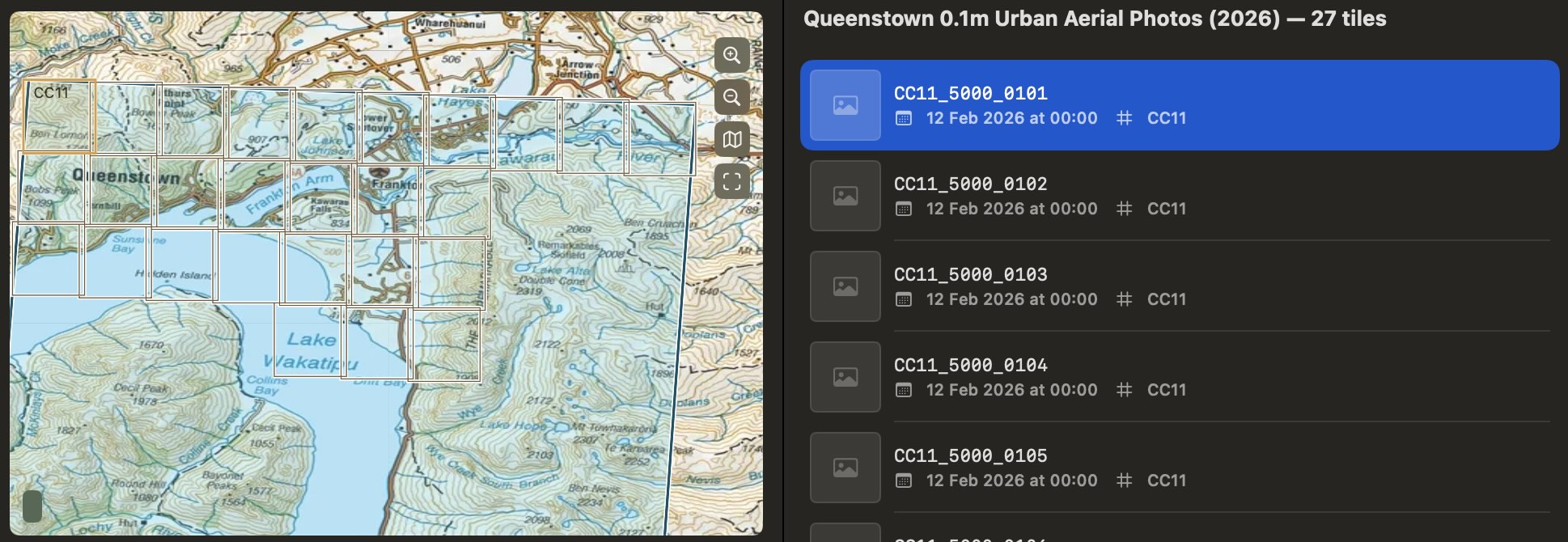
A chosen LINZ survey with its tile grid on the map, tiles selected and a download summary
Survey → tiles 93 tiles, 3 selected 460.5 MB map and list are one selection

Choosing a survey draws its tiles on the map, and the map and the list are one selection - click a tile on either. Hovering names the sheet the way LINZ printed it and the tile by its filename. The download states its size before it starts.

Downloads and failed transfers

Bands on different native grids are assembled as separate stacks and never resampled together. A file already on disk is not fetched again. A dropped transfer is retried and resumed where the archive allows it; the retry fetches only what is still missing, the partially written file is discarded - a truncated raster that looks openable is worse than an absent one - and the failed attempt stays on record as its own row. Landsat is free on Planetary Computer and requester-pays on Earth Search, and the panel says which before you commit.

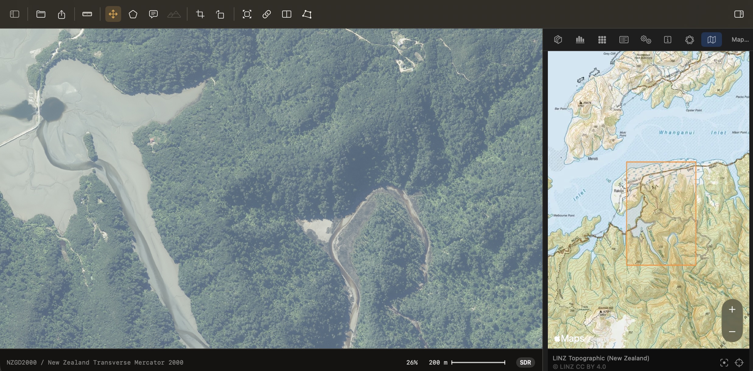
The Map Overview pane showing the national topographic basemap beside a scene
Inspector ▸ Map overview LINZ Topo50 where it exists Apple's basemap where no national service does

Once a scene is open, the overview pane answers “where is this?” against real topography. The source is picked by the ground under the scene, so New Zealand gets the LINZ 1:50,000 series and Switzerland gets swisstopo, while ground no national service covers falls back to Apple's map - dark, muted, points of interest off. That fallback was measured rather than assumed: over Aoraki it carries shaded relief, glaciers and landcover; over farmland it is very nearly blank, which is why it is the fallback rather than the preference. The scene footprint and your cursor are drawn on it, and any manual pan turns following off.

Composites& spectral indices

Composites and spectral indices

NDVI is (B08−B04)/(B08+B04) on Sentinel-2 and (B5−B4)/(B5+B4) on Landsat 8. You do not tell Hachure which is which - the catalogue carries every band's centre wavelength, FWHM, ground sample distance and spectral role, so the preset resolves itself against whatever stack is open. The same is true of NDWI, NDMI, NBR, NDSI, NDRE and tasseled-cap brightness, greenness and wetness.

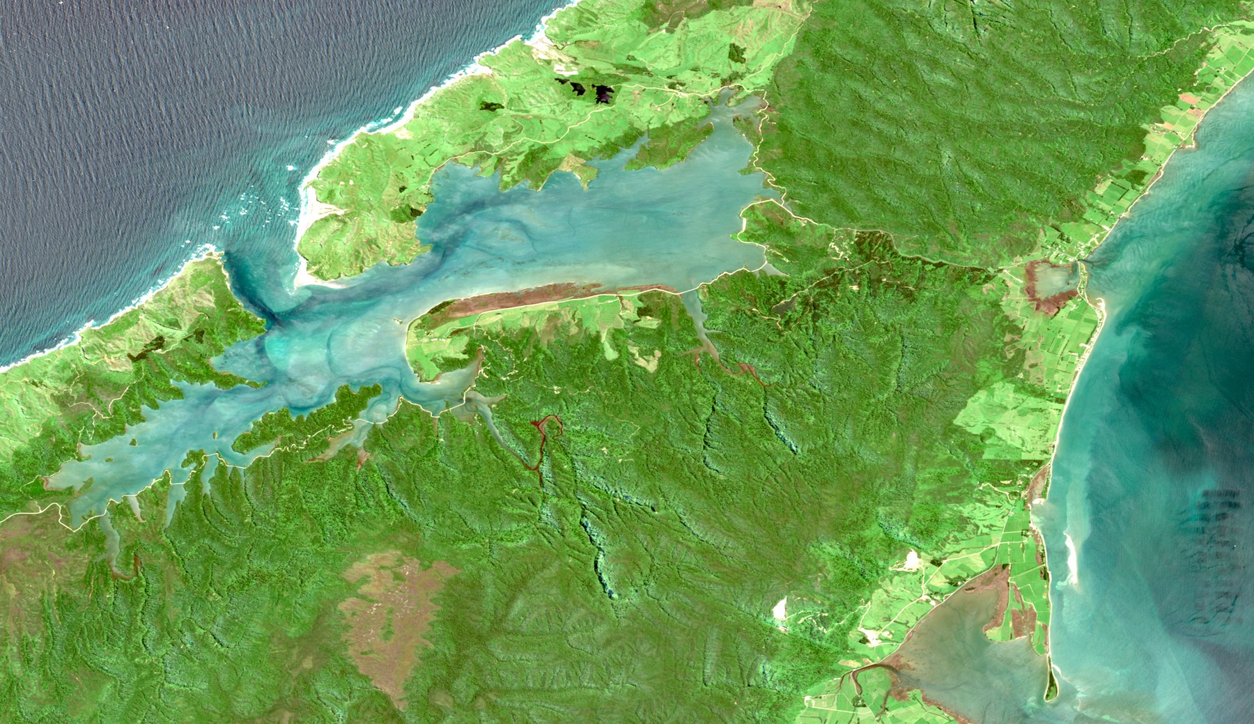
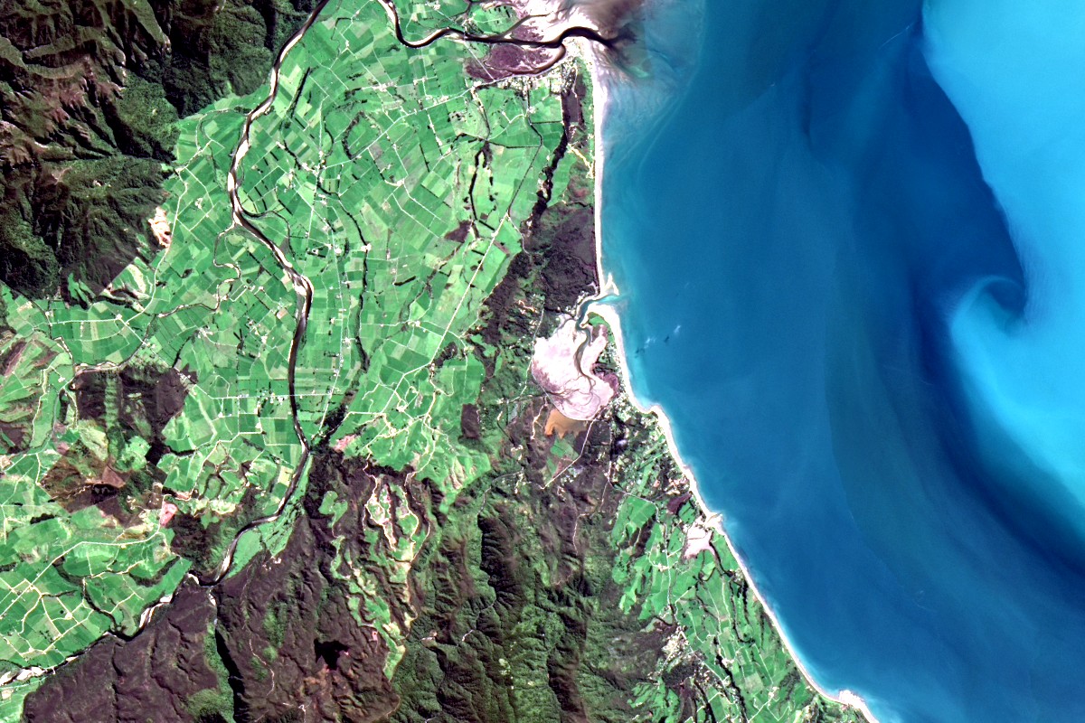
Sentinel-2 natural colour composite of Whanganui Inlet and Golden Bay, north-west Nelson.
Sentinel-2 L2A B04 · B03 · B02 10 m 2025-12-03 WGS 84 2438 × 1407
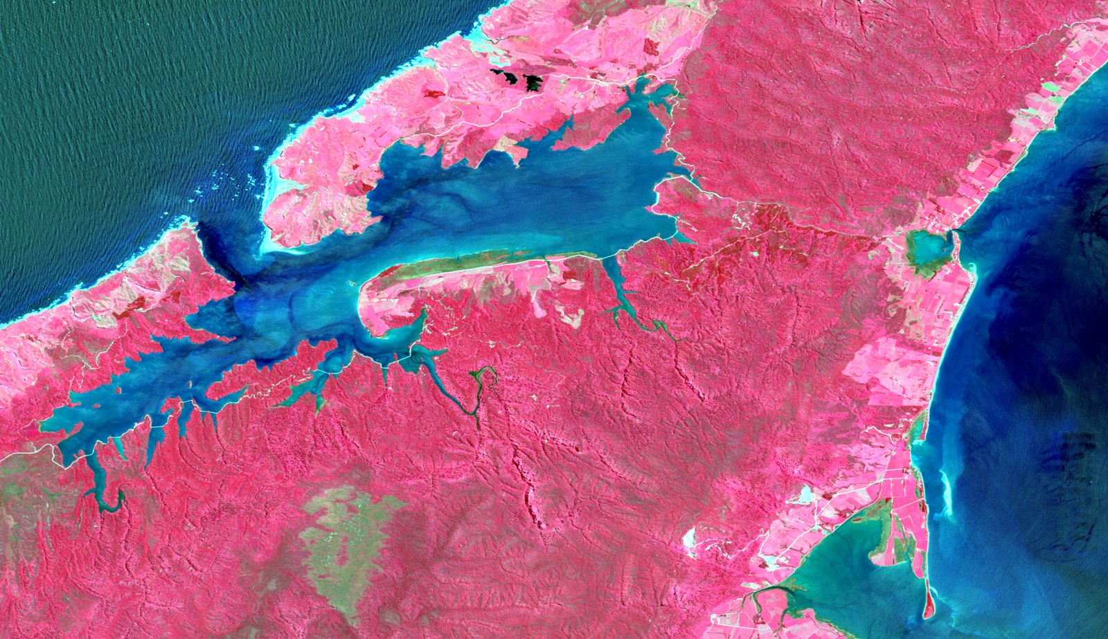
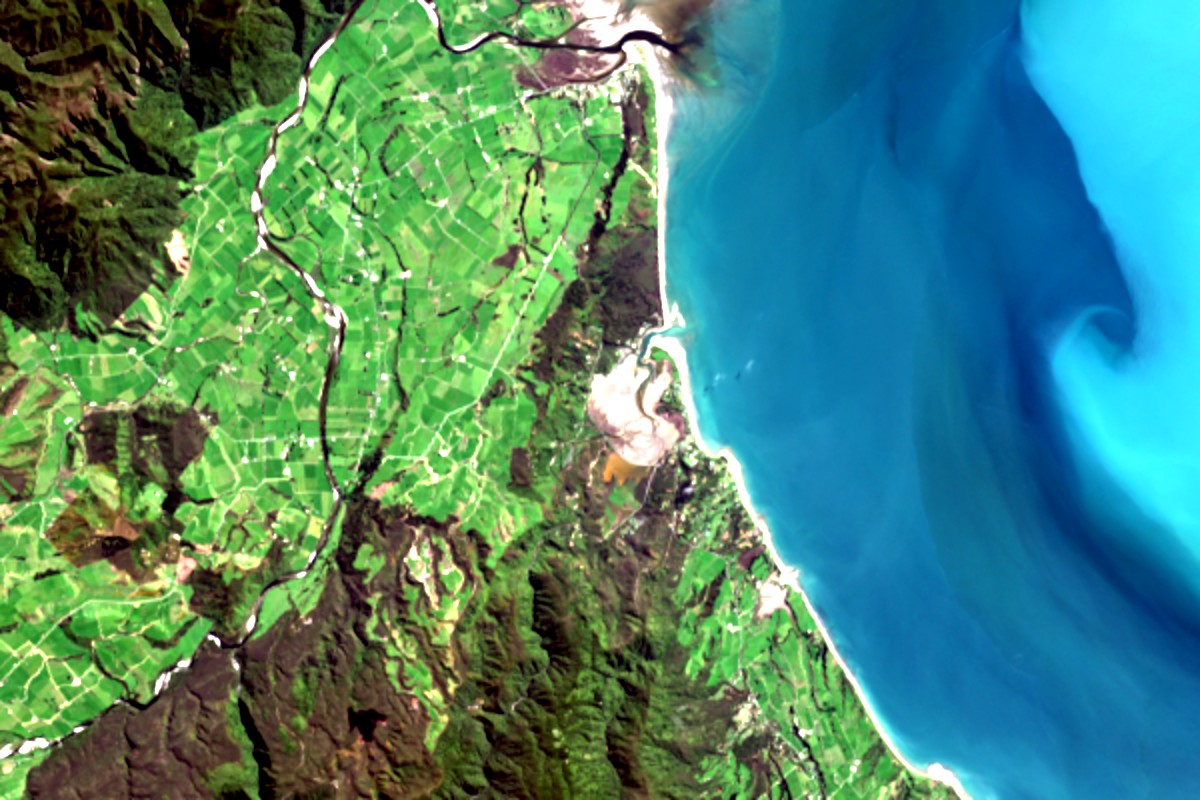
Colour infrared composite of the same Sentinel-2 scene, vegetation in red.
Colour infrared B08 · B04 · B03
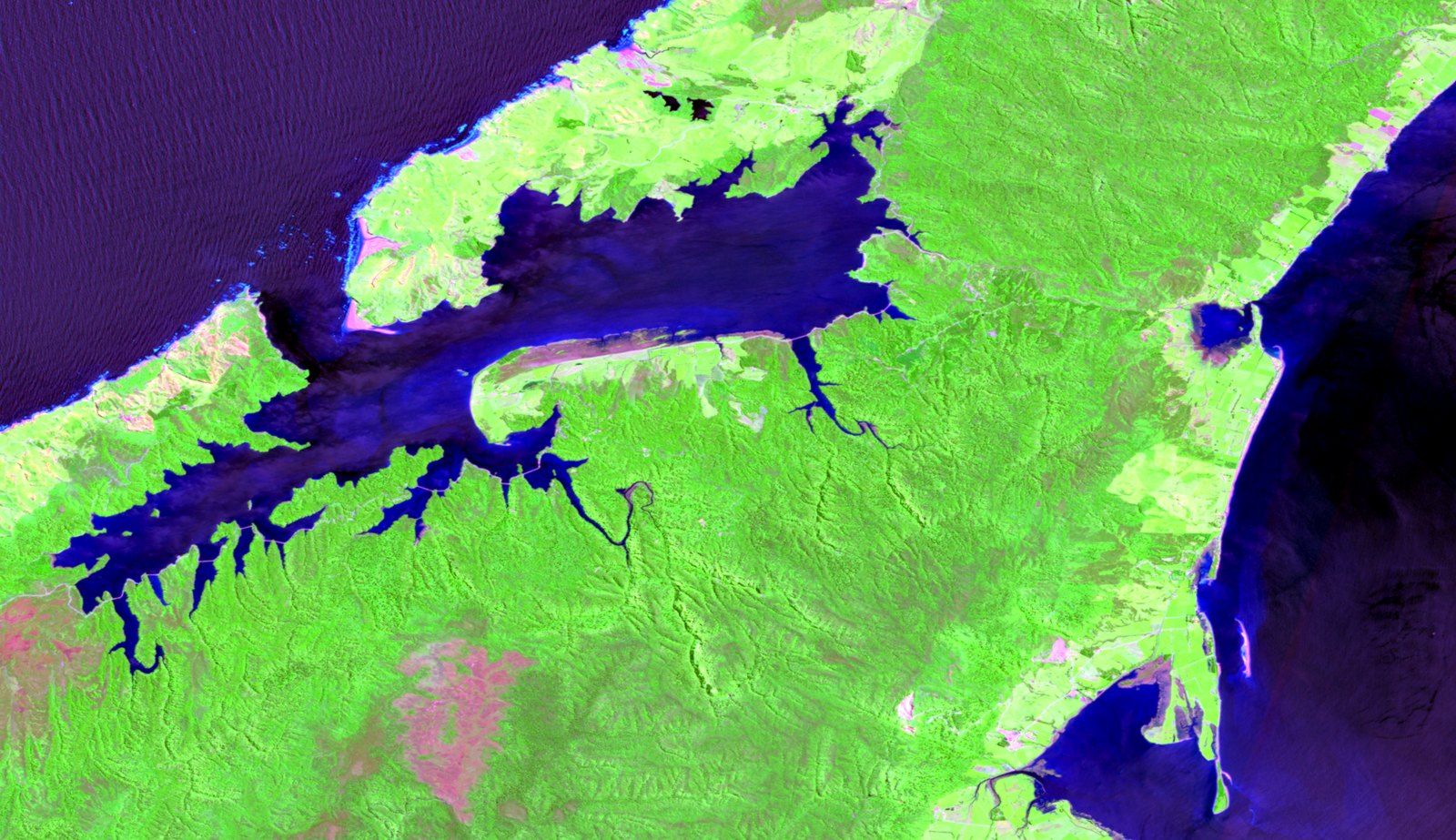
Short-wave infrared composite of the same Sentinel-2 scene.
Short-wave infrared B12 · B08 · B04
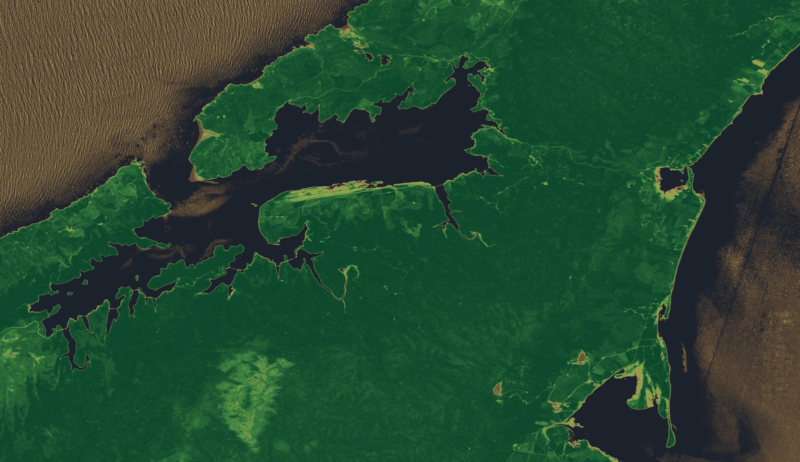
NDVI computed from the Sentinel-2 red and near-infrared bands.
NDVI −0.2 to 0.9
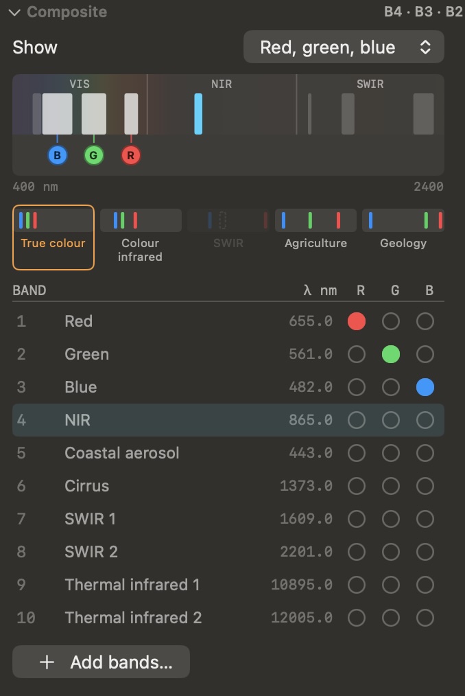
Inspector, Bands, Composite panel cropped to the panel: a wavelength axis from 400 to 2400 nm divided into VIS, NIR and SWIR with each band drawn as a passband, blue green and red pucks beneath the assigned bands, five presets drawn as the spectra they select, and a band list giving name, centre wavelength and channel assignment
Bands ▸ Composite 400 – 2400 nm

Band assignment on the spectrum

The Composite panel draws every band that states a wavelength where it actually sits, as a passband rather than a point, with a draggable puck per display channel. Centring one channel in an absorption feature and the other two on its shoulders is a drag along the axis - the workflow three band-number popups cannot express. The presets are drawn as the spectra they select, so you can see what a choice will do before you make it.

Bands with no stated wavelength still appear in the list below, fully assignable; they simply have no position, which is a fact about the file rather than a limitation of the panel.

A wavelength axis as an assignment control is established prior art; what is unusual here is making it the primary control, in the place bands are assigned, with bands drawn as passbands rather than points.

Spectral profile click a pixel value per band

Click a pixel and its full spectrum is plotted - value across every band, against wavelength where the bands declare one and band index where they do not. The y-axis is pinned rather than rescaled per pixel, so scrubbing across a boundary shows the spectrum changing instead of the axis jumping. On a hyperspectral cube that is the fastest way to tell two surfaces apart; on a ten-band stack it is the fastest way to catch a band assignment that is wrong.

Beyond the presets, a custom expression takes an arbitrary formula in b1…bN with arithmetic, comparison, logical and bitwise operators, conditionals, clamp, min and max, logarithms, safe division and QA bit extraction. One typed expression tree drives both the CPU evaluation that writes a Float32 GeoTIFF and the Metal shader compiled at runtime for the live view, and the two are tested against each other for parity - so the picture on screen and the file on disk are the same arithmetic.

Worth knowing An index is only as good as the spectral roles behind it. NDVI uses whichever bands are named NIR and Red; on a stack whose roles are wrong the arithmetic still succeeds and returns a plausible surface of the wrong two bands. The Composite panel is where you check, and the spectral profile is how you notice.

DisplayTone & fidelity

Display tone, and writing it into a raster

Stretch, gamma, curve and colour map are display exposure. Processing jobs, band maths and the GeoTIFF export read source samples regardless of what the screen is showing, so you can drive the display as hard as you like without wondering whether it has contaminated a result. Nothing is corrected on open: the default is the band's own full range. When you do want the curve in the file, one named command puts it there and labels what it made.

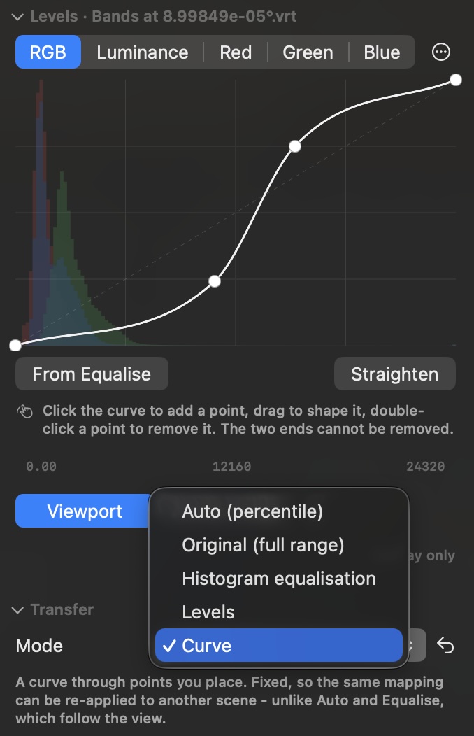
The Levels panel: a tone curve with control points drawn over the red, green and blue histograms of the data going in, with the transfer mode set to Curve
Levels ▸ Curve the curve sits on the histogram

Five transfer modes - full range, percentile, histogram equalisation, levels and a tone curve - and the curve is drawn over the distribution it is shaping rather than beside it, because the judgement being made is “steepen where the pixels are”. The histogram underneath shows the values going in and holds still as you drag: one redrawn from the output always looks well spread, which tells you nothing. A curve can be derived from an equalisation and then edited, and unlike Auto it is fixed, so the same mapping can be re-applied to another scene.

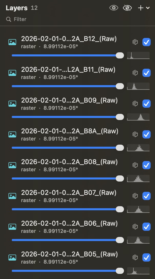
The Layers sidebar with several rasters, each row carrying its own value distribution drawn as a small sparkline
Layers a distribution per row

Each raster layer carries its distribution as a sparkline in its sidebar row, which is how you spot the one layer in a stack of twelve whose histogram sits somewhere different - before it turns into a mosaic seam or a bad difference. It is the question the Levels plot answers for one layer, asked of the whole stack at a glance.

Apply Display Tone Curves

Three exits, and the difference between them is what happens to the curve. Export as GeoTIFF writes the source's own samples and records the curve beside them - described, not applied. The rendered exports (PNG, HEIC, OpenEXR) apply it but produce a picture: a display composite with no georeferencing, 8-bit or Float16. Processing ▸ Radiometry ▸ Apply Display Tone Curves is the one in between, and the one an expert asking for a stretched product usually wants - the curve applied, the raster kept. Every display channel goes through its own transfer, whatever is in force, and the result is a georeferenced GeoTIFF at full bit depth: either the source's own data type spread over that type's whole range, which is what another GIS or a print expects to be handed, or Float32 holding the transfer's 0 to 1 output with no requantisation at all.

The curve is evaluated per sample, not sampled from the display's lookup table. The shader reads 4096 entries, which is sixteen times coarser than uint16 data, so going through it would quantise the written file down to whatever the screen happened to need. The file that comes out is finer than the display was, and its metadata says so. Where a contributing band declares nodata and the output is an integer type, zero is reserved for it and the tone occupies one level less - an integer band cannot hold NaN, and absent ground reading as legitimate black is the one confusion worth a level.

What the output says about itself A tone curve clips at both ends and is not invertible, so the result is not radiometry and cannot be treated as any. The file states that in its own metadata rather than leaving it to be remembered: a per-band description ending (not radiometry), and a tag reading “these samples are display intensities… the measurements are in the source named above” - along with the source path, the transfer used on each channel and a note of any clipping. Nothing about the display path changes: this is a transforming operation, chosen once, by name.

Extended dynamic range and colour management

A sixteen-bit scene holds far more range than a standard-dynamic-range screen can present, which is why so much of the craft of looking at one is choosing what to sacrifice. On a display with extended range there is less to sacrifice: the composite is rendered to rgba16Float in extended-linear Display P3 and handed to the compositor at that depth, so bright cloud tops and shadowed valley floor can hold detail in the same view rather than trading against each other in the stretch. Nothing along the way is quantised to eight bits.

It is opt-in, and it does not pretend. SDR is the default; headroom is read from the screen the window is actually on and re-read when it moves to another; and if that screen has no usable headroom the effective mode stays SDR even with HDR preferred, rather than rendering as though it were there. The footer says which regime you are in - a plain SDR or HDR badge - and the tooltip gives the number: rendering in HDR, output range 0 to 3.4× SDR white, or rendering in SDR, display EDR headroom 1.0× (no EDR). That matters when two people compare the same scene on different machines, and it is the sort of thing that is invisible until it has already misled somebody.

Colour is managed rather than assumed. The layer declares its colour space, so ColorSync converts to the profile of whatever display is attached instead of firing raw numbers at the panel - a wide-gamut composite looks the same on a calibrated studio display as on a laptop, and a colormap ramp is the ramp you chose rather than the one the screen happened to make of it. Exports stay SDR unless you pick HDR explicitly, and the export panel says so; OpenEXR is there for when the float range needs to leave the app intact.

Resolution and bit depth

Twelve- and sixteen-bit data stays at its own depth from disk to screen, and the display never invents a sample when it magnifies. A readout, a histogram bin and a percentile clip all refer to values the file actually contains. Decimation is allowed to sample, because the alternative is showing one pixel in nine; a raster with no overview pyramids opens anyway, streaming from full resolution, and a banner offers to build a sidecar in the background - mode resampling for thematic rasters, average for continuous ones.

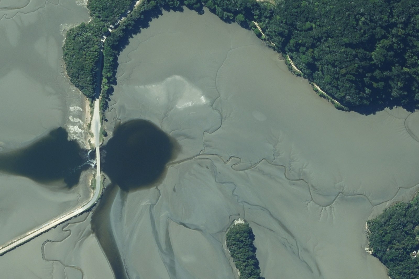
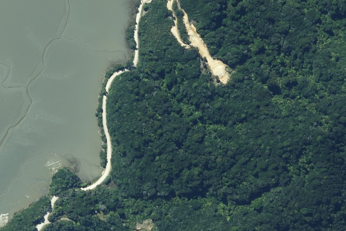
Tidal delta and causeway in 0.3 m colour aerial photography, north-west Nelson.
Aerial photography 0.30 m 1800 × 1200 source pixels NZGD2000 / NZTM2000 (EPSG:2193) Whanganui Inlet
A 600 by 400 pixel crop of the same aerial photograph, shown at exactly one screen pixel per source pixel.
1:1, no resampling 600 × 400 px = 180 × 120 m
Native bush, farm boundary and estuary margin in 0.3 m aerial photography.
Bush margin and tidal flat decimated for the page, not by the app

Polygons and processing regions

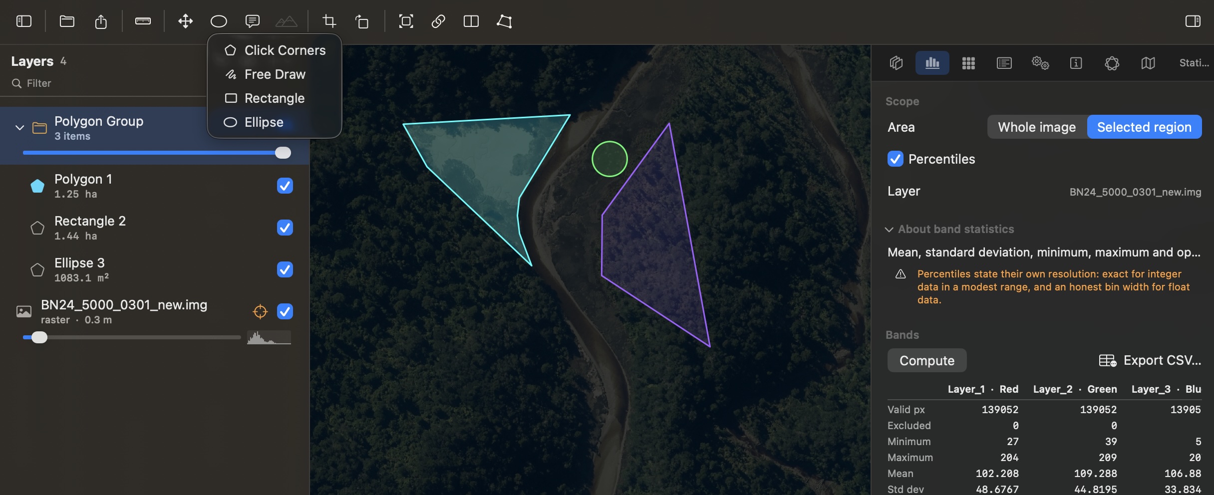
Click corners, free draw, rectangle or ellipse. Each finished shape becomes its own layer inside a polygon group, carrying its ground area in whatever unit suits its size - hectares for a paddock, square metres for a gravel bar - and a distinct tint, so overlapping regions stay legible. Mark one Use as Processing Region and it turns graticule cyan; every region-aware job then clips to it, and the Processing menu says which region it will use. An imported shapefile or GeoJSON boundary works the same way with no conversion.

The region is immediately the scope for measurement, not only for jobs. Band statistics switches between whole image and selected region and reports, per band, the valid and excluded pixel counts alongside minimum, maximum, mean and standard deviation - with percentiles that state their own resolution: exact for integer data in a modest range, an honest bin width for float. Zonal statistics does the same per polygon, in one pass however many zones there are, and the table exports as CSV.

Rectangle, ellipse and freehand polygons over a raster, one marked as the processing region
Polygon tools corners · free draw · rectangle · ellipse 1.25 ha · 1.44 ha · 1083.1 m² Statistics scoped to the selected region

RadiometryPhysical values

Calibration, atmospheric and topographic correction

Metadata ingest reads Landsat MTL, Sentinel-2 SAFE, Maxar IMD with RPB, Airbus DIMAP v2 and NITF, and records what calibration each delivery publishes without applying any of it. Run the conversion when you want it and the result carries the quantity, the units, the exact equation and which coefficient came from where - so a reflectance product can be audited a year later.

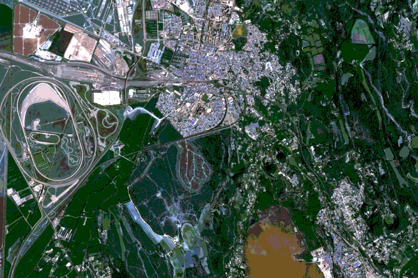
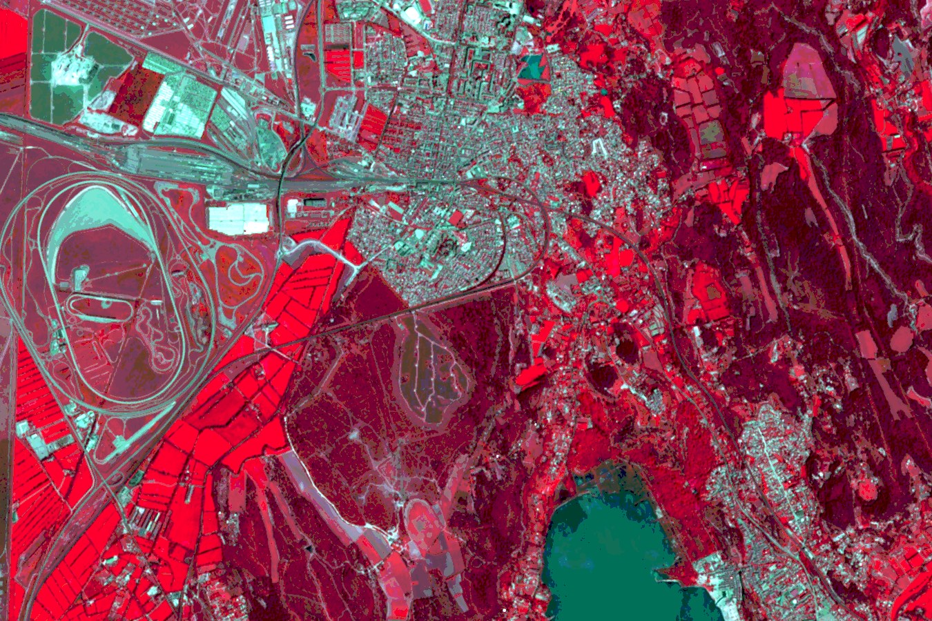
SPOT 6 multispectral scene in natural colour: farmland, a motorway interchange, a town and a lake.
SPOT 6 multispectral natural colour
The same SPOT 6 scene as a colour infrared composite.
SPOT 6 multispectral colour infrared

Calibration covers scale and offset in both conventions, solar-elevation reflectance, Planck brightness temperature, Sentinel quantification, Maxar gain and bandwidth, DIMAP divisor gain and lookup tables. Only the operations you tick are applied, results are Float32 and unclipped, and a fill value or an out-of-range input becomes NaN rather than a plausible number.

Atmospheric correction is per-band dark-object subtraction with the scene percentile and sample bound in your hands. It is labelled DOS rather than dressed up as 6S: it assumes somewhere in the scene is genuinely black in every band, which over a bright arid scene or a small subset is often false.

Topographic correction offers SCS+C, C-correction, Minnaert with the constant fitted per band, and the statistical-empirical rotation. Slope and aspect come from a Horn 3 × 3 operator on the DEM you choose; a correction fitted where the DEM does not reach is not applied there, and the report says how much of the scene was covered.

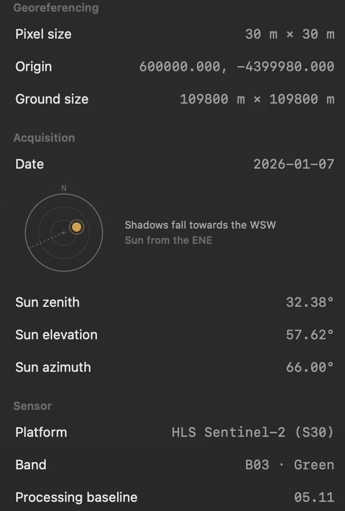
Inspector, Info, Acquisition: the sun-angle glyph drawing the scene's illumination as the sky dome seen from above, with the sun placed where the acquisition metadata puts it
Acquisition geometry drawn, not tabulated

Sun zenith and azimuth are auto-filled from acquisition metadata where the product states them, and the Info inspector draws them rather than only listing them: the glyph is the sky dome seen from above, with the sun where the metadata puts it, so a low winter sun and a near-nadir summer one are told apart at a glance. That matters because illumination geometry decides whether a topographic correction is worth running at all.

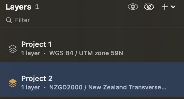
The Layers sidebar with layers grouped into projects by coordinate reference system, each group labelled with its CRS
Projects grouped by coordinate system

Layers that cannot share a grid are not silently piled together. They group into projects by coordinate reference system, each labelled with its CRS, so a NZTM survey and a UTM scene sit in separate groups until you reproject one - which makes “why will these not overlay?” a question you can answer by looking. A whole session, layers and all, saves as a project file and reopens as it was.

ChangeDrag the pane

Change detection and radiometric normalisation

The base document is A and any added or derived raster is B. Fixed side by side, a draggable swipe, a linear blend, and timed flicker - all display-only, all isolating A and B from the rest of the stack. Up to four named view groups link camera, zoom and crosshair across separate windows, in geographic coordinates where both datasets have a CRS.

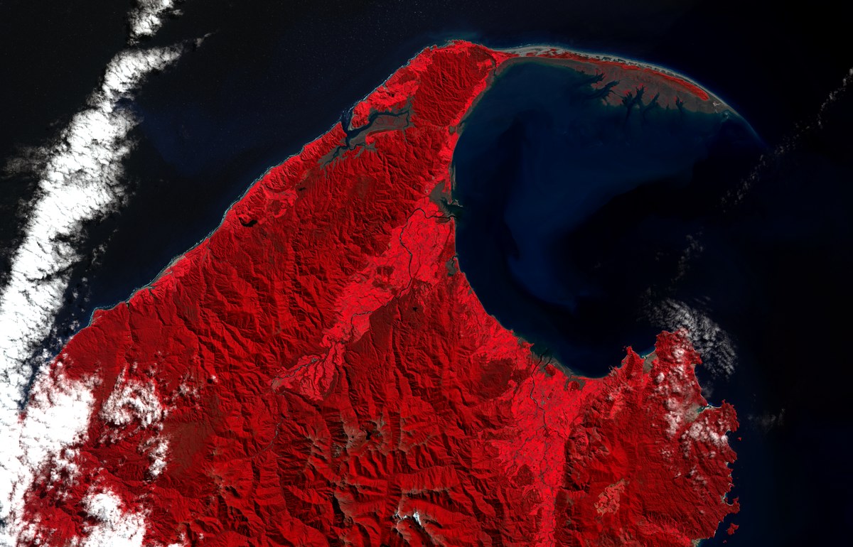
Landsat 8 colour infrared scene of north-west Nelson, September 2013.
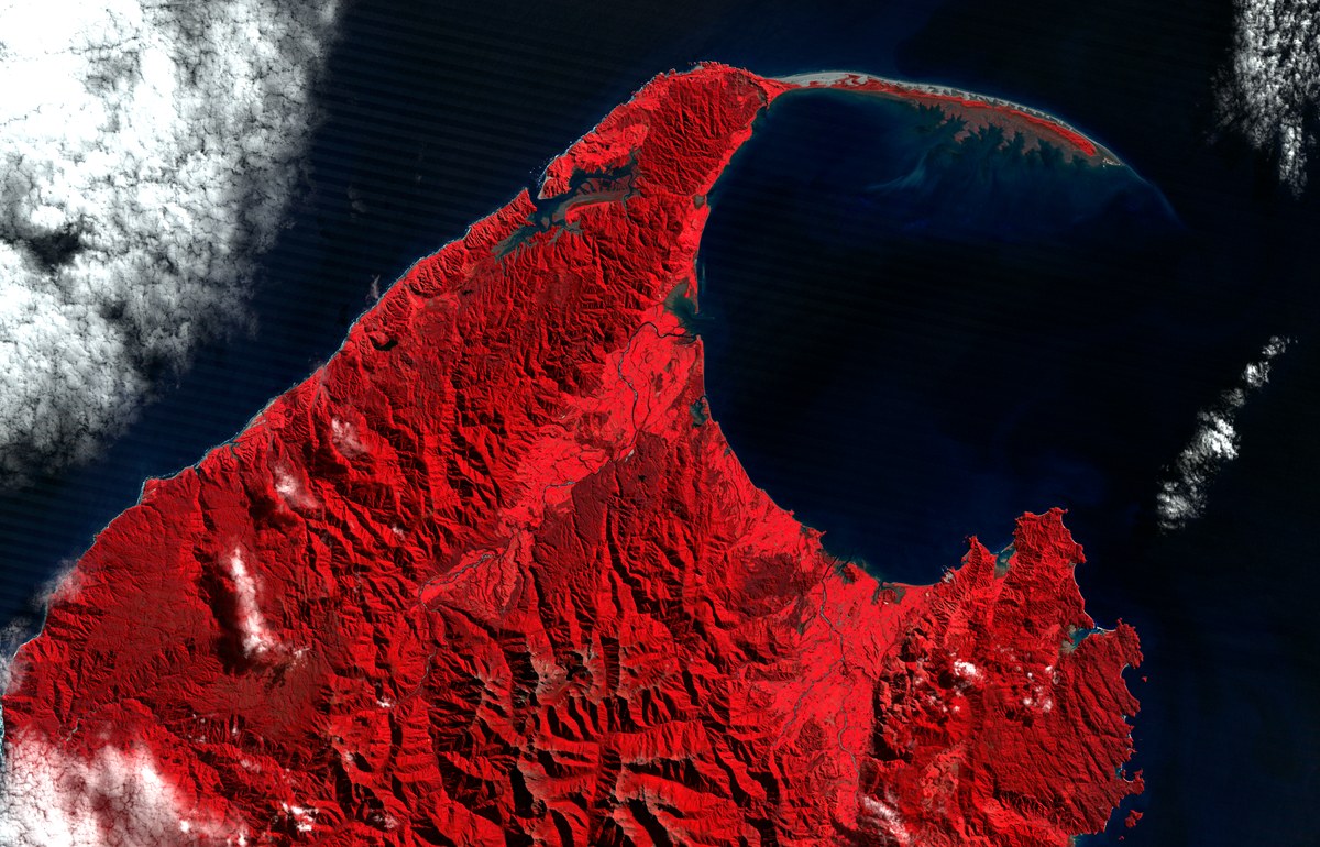
Landsat 4 Thematic Mapper colour infrared scene of the same ground, April 1989.
B · 1989-04-08 · TM A · 2013-09-25 · OLI
Landsat path 074 row 088 NIR · red · green 30 m UTM zone 59S the same 94 × 61 km window in both epochs

Change detection offers differencing, log-ratio for radar, index difference including dNBR burn severity, and IR-MAD's no-change probability as the threshold. Every method compares co-located pixels, so the panel states the same-grid requirement up front rather than failing halfway through a read - and it asks you to record what normalisation was done, because a change product that does not say gets believed.

Six ways to normalise: histogram specification, linear optimal transport matching mean and full covariance across bands, global regression, LIRRN, and IR-MAD. Accuracy assessment follows the good-practice area estimators rather than a single headline percentage, and reports quantity and allocation disagreement in place of Kappa.

TerrainSame ground as the hero

Relief shading, slope, profiles, elevation change

Relief shading, the slope raster and the topographic correction all use Horn's 3 × 3 kernel, which means a slope class and a hillshade cannot tell you different things about the same cell. Shading stays display-only: every control has a live thumbnail, and the full-resolution pass runs only when you press Apply, arriving as its own layer. Slope writes a file - degrees, percent or rise over run, with the downslope bearing beside it if you want it.

The illumination dial the sun on the sky dome

The light is placed on a dial rather than through two numeric sliders - bearing around the ring, height from the centre - because that is the shape of the quantity, and finding the azimuth that reveals a lineament is a matter of moving the sun until it does. Multi-directional light, cast shadows, skylight and a hypsometric, slope or aspect tint over any colormap are all there.

The shading is deliberately not exportable as a raster, because it is a picture and the slope raster is the measurement. Both come from the same operator, so the two cannot disagree about a cell.

Relief shading, applied 1 m LiDAR · 6 lights · cast shadows arrives as its own layer
Multi-directional hillshade with hypsometric tint of a 1 m LiDAR surface, showing spurs, gullies and individual tree crowns.
LiDAR surface model 1 m posting multi-directional shading, hypsometric tint 1800 × 1200 m NZTM2000
Slope raster of the same surface, colour-mapped from flat to fifty degrees.
Slope 0 – 50° Horn 3 × 3
The identical ground photographed at 0.3 m: bush-covered spurs, pasture on the terrace and the estuary margin.
The identical ground 0.30 m aerial

Elevation profiles

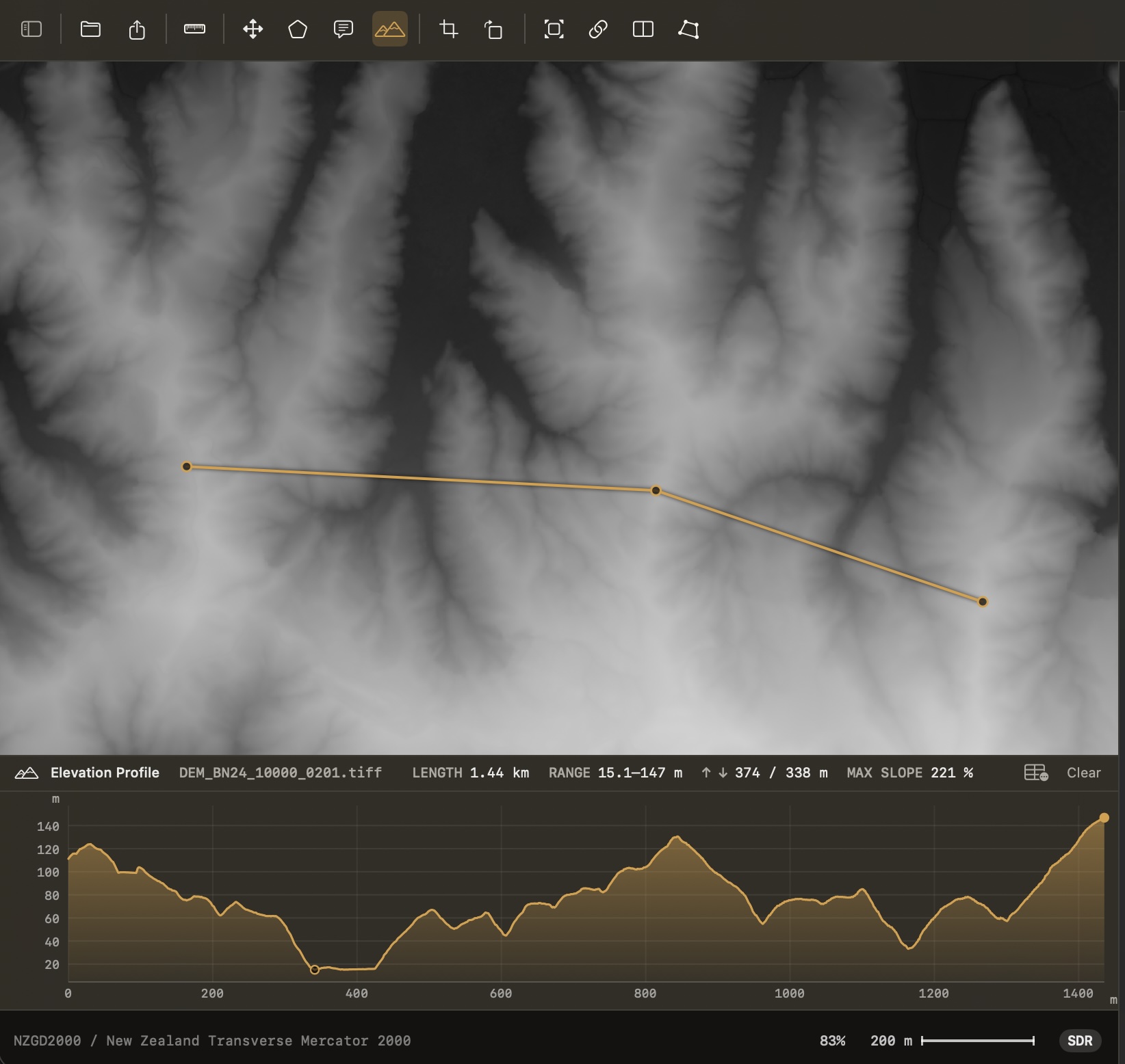
Click a line across an elevation surface and the terrain profile charts as you go - length, elevation range, ascent and descent, and maximum slope. Where the line crosses ground the elevation model does not cover, it reports the count of those cells rather than drawing a line through them. It sits in a pane above the footer rather than floating over the map, so the ground being measured stays visible while it is being measured, and the table glyph beside the readout takes the samples out as a file.

A three-vertex profile line drawn across a greyscale elevation model, with the cross-section pane beneath reporting length, elevation range, ascent, descent and maximum slope
Elevation profile 1.44 km range 15.1 – 147 m ↑ 374 / ↓ 338 m max slope 221 % NZGD2000 / NZTM2000

A slope is a height over a ground distance and most DEMs state only the second. The ground distance comes from the geotransform, converted per axis on a geographic grid because a degree of longitude shortens with latitude; the vertical unit comes from the band or a compound CRS, and where nothing declares one the panel says the heights were taken as metres. A DEM in feet read as metres reports every slope 3.28 times too steep and fails in no way at all - which is why the panel says it rather than assuming you knew.

DEM of Difference reports volume lost and gained with the uncertainty that makes the figure defensible: a level of detection measured from ground you mark as stable, a probability of real change per cell, and a spatial-coherence pass that keeps a coherent patch of marginal cells and drops isolated spikes. Co-registration is offered as a check and stays off, because a rigid vertical correction removes a constant offset and uniform soil loss is a constant offset. InSAR displacement answers the neighbouring question - millimetres of motion along one line of sight at 30–80 m posting, with the coherence that says which cells are a measurement at all.

FusionDrag the pane

Pan-sharpening and resolution fusion

SFIM detail injection, Brovey, GSA - Gram-Schmidt Adaptive, which fits its intensity component by least squares instead of assuming a flat band mean - and MTF-GLP-HPM, which degrades the guide through a Gaussian matched to the sensor's modulation transfer before injecting it. Method, guide band, coarse resampling kernel and detail amount are all yours to set.

Landsat 8 natural colour fused with the 15 m panchromatic band, showing paddock boundaries and river channels.
The same Landsat 8 natural colour bands at their native 30 m posting.
B · 30 m multispectral A · fused with 15 m pan
Landsat 8 OLI B04 · B03 · B02 guided by B08 2013-09-25 18 × 12 km, Golden Bay

MTF-matched and GSA hold a property you can test: aggregate the fused result back to the coarse grid and it should reproduce the input. A plain component substitution does not hold it nearly as well. So where a figure has to be defensible per pixel - a calibrated reflectance, an index quoted as a number - compute it on the source bands and use the fused product for geometry. Only layers finer on the ground than the target are offered as a guide; it streams one band at a time, so peak memory does not scale with band count.

ClassificationAnd what follows it

Classification, and its diagnostics

Unsupervised: K-Means with k-means++ and maximin seeding, ISODATA with adaptive split and merge, and a Gaussian/Mahalanobis mixture - all deterministic, all multicore, with a Metal backend for the assignment step, and images too large for memory fitted on a decimated sample and assigned block by block. Supervised: random forest, maximum likelihood, minimum distance and spectral angle from training polygons you label.

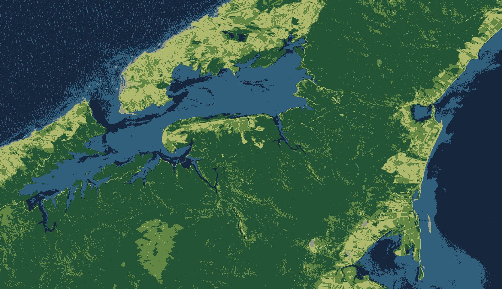
Six-class unsupervised classification of the Sentinel-2 scene: deep water, estuary, bare ground, native forest, scrub and pasture.
Unsupervised classification k = 6 blue · green · red · NIR · SWIR1 · SWIR2 Sentinel-2 L2A, 10 m
Separability before you trust the classifier
Reclassify breaks over the distribution

Two classes that overlap in feature space cannot be told apart by any classifier, so separability is drawn as a heat map before you commit: the problem pair is a dark cell you notice, rather than one number among thirty in a table. The panel is also explicit that out-of-bag accuracy is not an accuracy assessment - it shares the training polygons' spatial autocorrelation - and the live preview fits on the visible extent, which makes it a tool for choosing k by looking rather than the model the full scene gets.

Reclassify turns a continuous band into named classes by a table of breaks, with the band's own distribution drawn behind them - because where a threshold falls is the whole of what the output says, and a number typed with nothing behind it is chosen blind. A value outside every class is left unclassified rather than pushed into the nearest one: clamping would let a top break typed as 3.6 instead of 36 report a whole property as the steepest class, complete and confident, with no gap anywhere to notice.

Land Resource Inventory intersects up to five factor layers - rock type, soil, slope, erosion, vegetation - into inventory units, sieves them to a minimum mappable area, and looks each combination up in an editable rule table for a Land Use Capability class. The class comes from the most limiting factor rather than an average; a factor nobody assessed leaves its units unclassified rather than optimistic; and a severity of zero, meaning somebody looked and found nothing, stays separate from nobody having looked. Every unit's row carries where each of its five statements came from.

MosaicJoining scenes

Mosaicking: seams, joins, balancing

The panel plans the output grid, reports overlaps and disconnected pieces, and pre-flights CRS, resolution ratio, overlap sufficiency and radiometry. Two seam solvers - least-cost path routed through waypoints you pin, and graph cut, which can isolate an island. Four join modes: hard, feathered on a linear or cosine ramp, distance-weighted, and seamless multi-band Laplacian.

Mosaicking live preview on a decimated grid seam editable by hand per-scene gain solved across every overlap at once

The preview composites on a decimated grid so the seam can be dragged and re-routed at interactive speed, and the cost surface behind it is a superset of the usual difference term: absolute difference plus gradient, constrained by a dilated mask. Radiometric balancing solves a per-scene gain and offset across every overlap simultaneously rather than chaining pairwise fits, which is what stops error accumulating along a strip.

Hard blending leaves values untouched and is the default; feathered, weighted and multi-band blending all rewrite pixels near the seam, and balancing rewrites whole scenes - so the panel says which of those you have asked for. The case it is built for is the large one: seventeen 0.3 m aerial tiles onto a single 32,000 × 60,000 four-band grid, 7.68 billion samples planned, composited and written in 62 seconds.

ProximalBelow the surface

Proximal survey, logger file to 3-D model

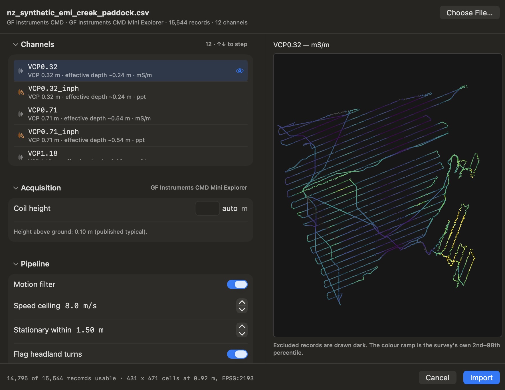
Point a logger export at Hachure and it recognises the instrument, works out the coordinate format, names each coil with the effective depth its separation gives, and produces three georeferenced products in one window: the measured points, an interpolated surface per channel, and an inverted conductivity-against-depth stack.

The Import Proximal Survey panel: the instrument recognised as a GF Instruments CMD Mini Explorer with 15,544 records over 12 channels, each coil named with its effective depth, an acquisition section carrying coil height, a pipeline of filter stages, and the survey traverse drawn live and coloured by the selected channel
File ▸ Import Proximal Survey GF Instruments CMD Mini Explorer 15,544 records · 12 channels 14,795 usable 431 × 471 cells at 0.92 m · EPSG:2193 synthetic test paddock

The panel is a stack of stages rather than a wizard: every filter is a row that switches off, each with its own numbers on show - motion filter with a speed ceiling in metres a second and a stationary threshold in metres, headland turns flagged - the pipeline re-runs on any change, and excluded records stay drawn in dark so you can see where a filter bites before you commit. Stages run in order: parse and project, acquisition geometry, motion filter, range filter, ferrous interference, along-track despike, rolling mean, GNSS latency, sensor offset, instrument drift, temperature standardisation to 25 °C, calibration against reference profiles.

It also shows its working. The instrument is identified from the file rather than asked for. Each channel is named with the effective depth its coil separation gives, so VCP0.71 reads as 0.54 m rather than as a number you have to convert. Coil height above ground - which every forward model needs and most exports omit - is filled from the published typical for the recognised instrument and labelled as that, not presented as measured. And where the coordinate format has to be inferred, the panel states the inference and the evidence for it: values exceed ±90°, integer parts are four digits wide, values carry a hemisphere letter.

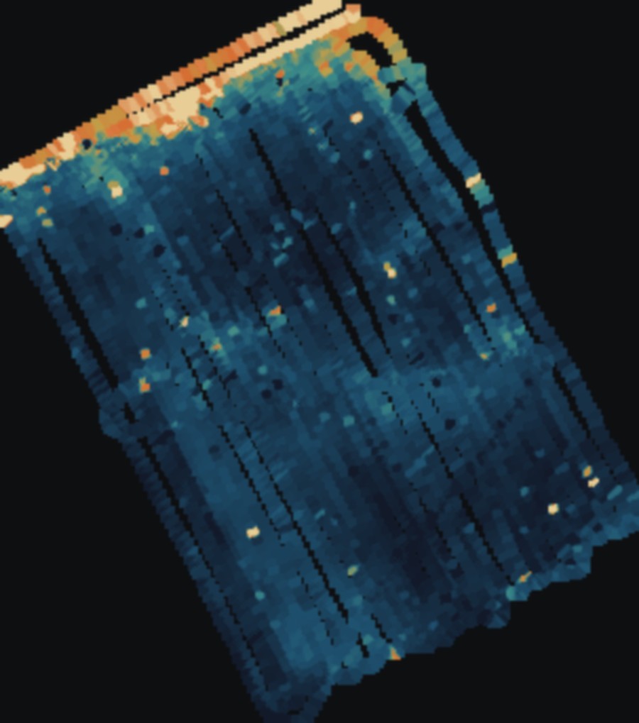
Interpolated apparent electrical conductivity from the shallowest coil, showing traverse lines and a conductive headland.
ECa, HCP 0.20 m ≈ 0.3 m effective depth open six-coil survey
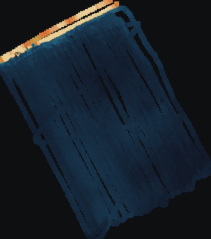
Interpolated apparent electrical conductivity from the deepest coil over the same survey block.
ECa, HCP 1.50 m ≈ 2.3 m effective depth same block, deepest coil
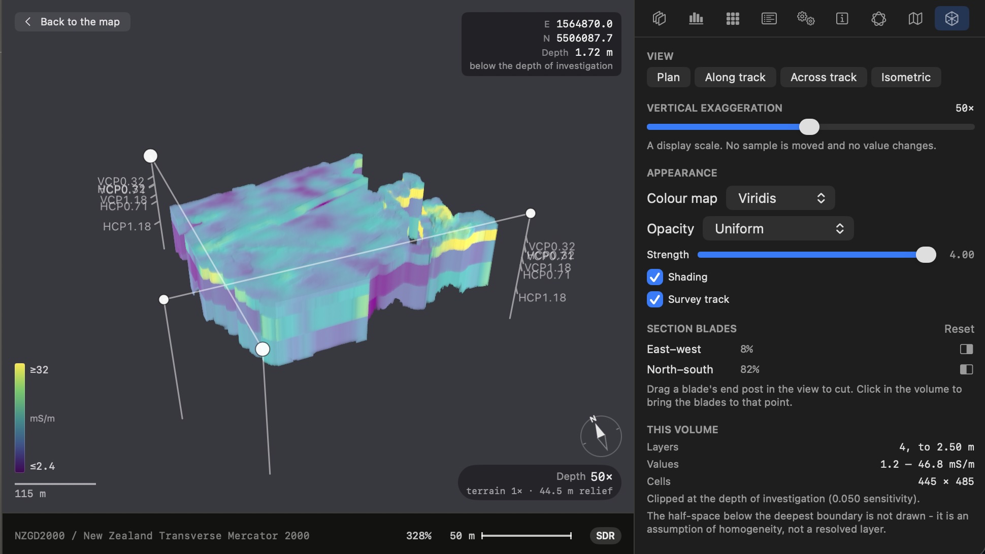
The inverted conductivity volume drawn in three dimensions and draped on the terrain, cut open by two section blades, with the coil depths labelled down both axes, a probe readout giving easting, northing and depth, a compass, a scale bar and the vertical exaggeration on screen
View in 3D 4 layers to 2.50 m 1.2 – 46.8 mS/m 445 × 485 cells blades cut at 8 % and 82 % depth 50× · terrain 1× · 44.5 m relief

The inverted profile is a volume, so it is drawn as one - ray-marched, draped on the terrain rather than laid out flat, with the coil depths labelled down both axes and two section blades you drag in to cut the block open. Probe it and the readout gives easting, northing and depth, and says below the depth of investigation when that is where you are pointing. The exaggeration factor stays on screen rather than hiding in a menu - both figures, the depth stretch and the terrain's own - because people misjudge layer thickness on an exaggerated view and an unlabelled one is actively misleading. The chrome is achromatic throughout: furniture borrowing a colour from the transfer function would read as data. And the block stops where the data does, clipped at the depth of investigation, with a line saying the half-space below the deepest boundary is not drawn because it is an assumption of homogeneity rather than a resolved layer.

Sounding Posterior exists because a misfit is not a resolution: it says the model reproduces the readings, not that a quite different model would not have done equally well - and for EMI one very often would. Sampling the posterior under a single sounding gives the width of each layer's credible interval, and past a factor of ten the data do not resolve that layer at all. Substrate Units then clusters the whole inverted column rather than a depth slice, segmenting first so the units come out spatially coherent, and ranking them against the handbook's coding turns them into an inventory factor layer.

ProcessingJobs, not filters

Every operation is a cancellable, budgeted job

Nothing blocks the viewer, nothing mutates the source, results arrive as new layers with their own provenance. Any whole-image job checks a memory ceiling before reading a pixel, so an over-large job fails in a second instead of paging for twenty minutes - and offers to run anyway, with the required and available figures on screen.

Radiometry

  • Radiometric Calibration DN → radiance / reflectance / BT
  • Atmospheric Correction dark object, labelled DOS
  • Apply Display Tone Curves curve into a raster, full bit depth

Geometry

  • Reproject kernel explicit
  • Resample to Match Layer exact grid
  • Subset Bands / Extent no interpolation
  • Ground Control Points affine · poly 1–3 · TPS
  • Pan-sharpen / Fuse SFIM · Brovey · GSA · MTF-GLP-HPM
  • Orthorectification RPC or GCP, with a DEM
  • Image-to-Image Co-registration GPU phase correlation
  • Topographic Correction SCS+C · C · Minnaert · rotation

Filters

  • Destripe FFT notch or row profile
  • Low-pass FFT or Gaussian
  • High-pass signed residual or high-boost
  • Sharpen unsharp · guided · Richardson–Lucy

Mosaic

  • Mosaicking least-cost or graph-cut seam
  • Normalise to Reference 6 methods incl. IR-MAD

Analysis

  • Band Math indices and expressions
  • Band Statistics per band, per region
  • Zonal Statistics one pass, any zone count
  • Principal Components / MNF noise-whitened
  • Change Detection diff · log-ratio · dNBR · IR-MAD
  • DEM of Difference volume with a level of detection
  • InSAR Displacement metres, with coherence
  • Slope degrees · percent · rise/run
  • Reclassify breaks → class raster + table
  • Land Resource Inventory five factors → LUC class

Classification

  • Classify K-Means · ISODATA · Gaussian
  • Supervised Classification RF · ML · min distance · SAM

Proximal survey

  • Plan Soil Pits ranked, by purpose
  • Substrate Units segment, then cluster
  • Rank Substrate Units → inventory factor layer
  • Sounding Posterior credible interval per layer
Processing menu seven groups a command that cannot run says why, in the menu

Nothing is greyed out in silence. Slope reads “is not an elevation model” against the layer it was asked about; Rank Substrate Units reads “run Substrate Units… first, then select its output”; a capability that is declared but unbuilt reads “not built yet”. The header states the processing region every region-aware job will actually use, which is the union of the polygons you selected and any vector layer flagged as a region - not a guess.

Job progress and derived layers

Long jobs report progress and cancel cooperatively; the Jobs inspector lists what has run and how long it took. Results are written to temporary files and opened as layers, which is what makes the menu feel immediate - so closing a window lists any derived layer you have not saved, with a format for each, and offers Save, Don't Save or Cancel. The formats are all scientific containers: GeoTIFF, Cloud-Optimised GeoTIFF, KEA and ERDAS Imagine.

Nothing is thrown away quietly on close, and on quit
Inspector ▸ Apple Intelligence on device answers shown with the catalogue rows behind them

Apple Intelligence

A question box over a journal of this session's questions and answers. Ask what wavelength Sentinel-2's B04 sits at, which bands make a colour-infrared composite of the scene that is open, what NDRE is computed from on this sensor, or where the pan-sharpening command lives and what its methods differ on. It runs on device, and the journal lives only as long as the window - nothing is written to disk, because these are working notes about somebody's imagery and a log that outlived the session would be a store of them nobody asked for.

What makes it usable rather than merely fluent is that it is not allowed to answer from recollection. Two lookups back it: the sensor catalogue, for exact band wavelengths, widths, ground sample distances, spectral roles and index formulas; and a written guide to the interface, for where a control is and what it does. The model is instructed to quote what it was handed rather than paraphrase it, and when the catalogue does not hold something it says so and lists what it does hold - because a wavelength wrong by 8 nm looks exactly like one that is right, and a plausible menu path is worse than no answer at all. Every answer is shown with the facts it was built from underneath it: not decoration, but the difference between a number you can use and one you have to go and check.

It is handed a value describing the open scene's metadata - sensor, acquisition, bands, CRS. There is nowhere in that type to put a pixel, so “the assistant does not read your data” is a property of the code rather than a promise about it. Where Apple Intelligence is unavailable on the machine, the panel says which reason applies instead of silently doing nothing.

ThroughputTime to a result

Whole-job timings, on stated hardware

The figures below are whole jobs on real scenes - open, read, compute, compress, write - not kernels timed in isolation, and nothing prepared beforehand and held outside the clock. The rate is megabytes of image data a second: source samples at their own width, which is what the algorithm actually reads, rather than bytes off disk, which moves with the codec. All of it was measured on one machine: a MacBook Pro with an M5 Pro, 18 cores and 64 GB of unified memory, release build. Treat them as a sense of scale rather than a specification.

Unsupervised classification

198MB/s

ISODATA over 553 megapixels and five bands on the Metal backend, end to end in 14.0 s: fit, assign every pixel, write the class raster and its attribute table. K-Means 219 MB/s, Gaussian mixture 187 MB/s.

Seventeen-tile aerial mosaic

124MB/s

Seventeen 8000 × 12000 four-band tiles at 0.3 m onto one 32,000 × 60,000 grid - 7.68 billion samples planned, composited and written in 62.1 s.

Sharpening, guided

796MB/s

4096 × 4096 × 3 Float32 in 0.253 s, reaching 10.5 of 18 cores. Richardson–Lucy at twelve iterations on the same raster: 278 MB/s.

Relief re-shade

124MB/s

34.6 megapixels of Float32 elevation in 1.11 s. The horizon field is a GPU march computed once per surface; moving the sun after that re-shades at this rate.

Is a minute fast? There is no directly comparable published figure, so this is a sense of scale rather than a benchmark. The nearest recent work - Nie, Cui & Wan, Remote Sensing 2023 - mosaics 48 Landsat-8 scenes, 55.28 GB across two UTM zones, on a Spark cluster of five blade servers: six-core Xeons, 32 GB each, 24 executor cores in total, 16 GB of Spark worker memory and 2 GB per executor. Their speed comparisons are against their own MPI and Spark baselines; ENVI appears in that paper as the quality reference, mosaicked for RMSE and SSIM, not as a speed baseline.

Their throughput is volume divided by “the running time of the mosaicking algorithm”, and the paper does not say whether blocking, HDFS ingest and the UTM to EPSG:4326 reprojection sit inside that time - the reprojection is described as done before the experiment, so probably not, which makes any rate taken from it a partial-pipeline number. The figure above is the other kind, and it is the write that bounds it: the mosaic reaches only 1.27 of eighteen cores, because compositing finishes far ahead of a writer that is single-threaded by design. Take from the comparison what it can carry - the hardware published work has needed for this job - and not a ratio.

Memory and streaming

Whole-image jobs stream in bounded blocks, so a raster larger than RAM is a longer job rather than a failed one. Before any of that starts, the job checks a memory ceiling you set - so an over-large run fails in a second with the required and available figures on screen, instead of paging for twenty minutes and then failing anyway. Reads take one GDAL handle per worker, because GDAL datasets are not thread-safe, and tiled output is what makes out-of-order block writes safe.

Every material job writes its own provenance into the result: the operation, the equation, the coefficients and which file the measurement belongs to. A topographic correction reports how much of the scene the DEM actually covered; a co-registration reports RMSE and peak ratio before and after; a DEM of Difference reports its level of detection. Results arrive as new layers and never overwrite a source.

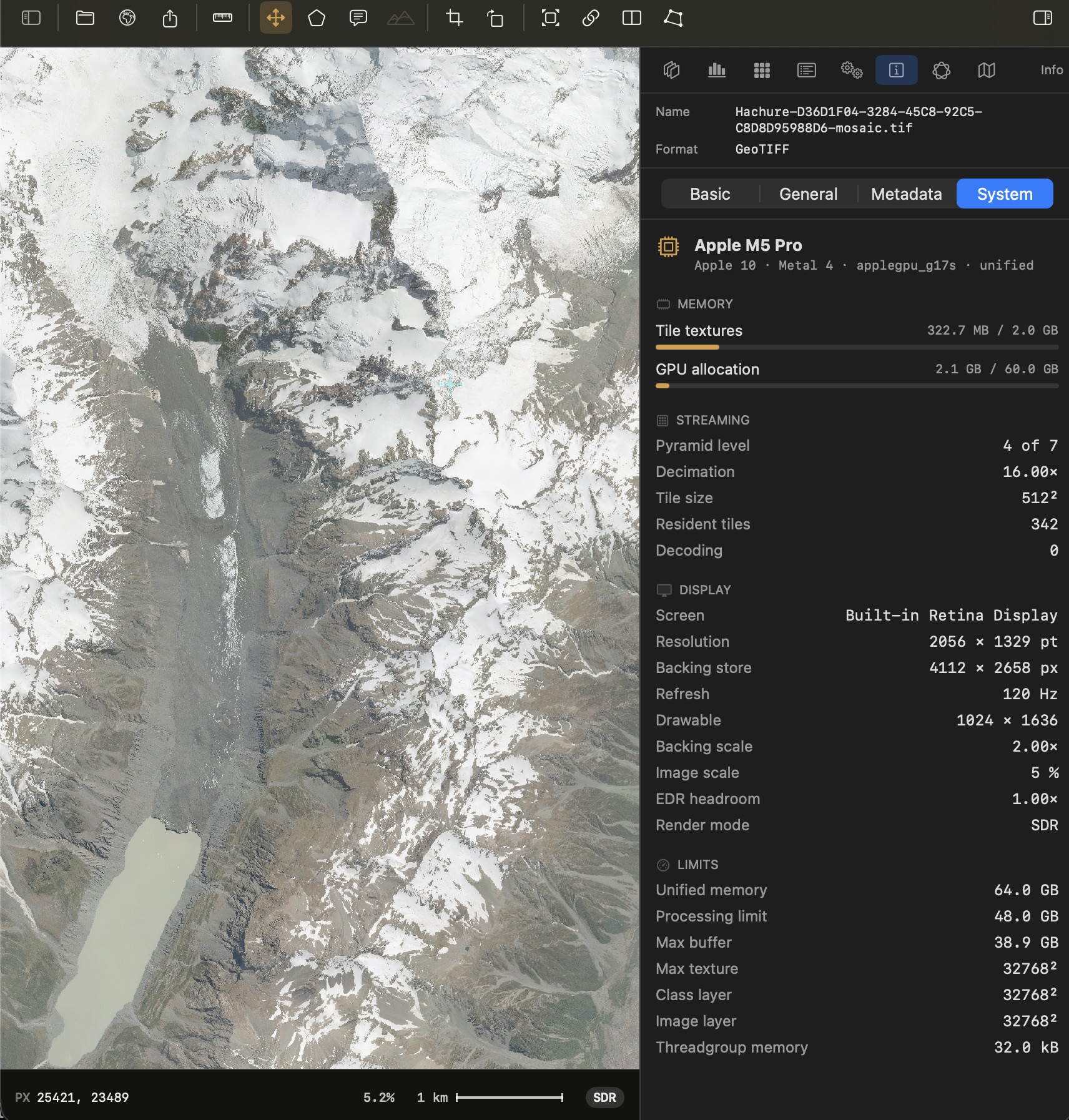
Inspector ▸ Info ▸ System

Inspector ▸ Info ▸ System is the instrument on the instrument. It reports the GPU and its Metal version, unified and GPU memory, the processing ceiling you set, and - the useful part while you are working - the live streaming state: tile size, resident tiles, tile-texture memory, which pyramid level is being drawn and how many source pixels that level is putting into each tile pixel. Beside it sit the display facts that change what you are seeing: screen resolution, backing scale, drawable size, refresh rate, render mode and EDR headroom.

That turns two vague complaints into answerable questions. Why is this scene soft? - because the pyramid level in use is decimating eight source pixels into each tile pixel, and zooming further will fetch the finer level. Why did that job refuse? - because the processing ceiling is set to half of 64 GB and the job wanted more, which the panel shows against the figure it was measured with. It is also the first place to look when a raster streams slowly: resident tiles climbing while tile-texture memory sits at the cache ceiling is a different problem from decode never finishing.

Inspector ▸ Info ▸ System live what the renderer is holding, and at which pyramid level

Interaction, and what it is built on

Band assignment, stretch, index maths and relief shading are evaluated on the GPU at full resolution, so changing what you are looking at is not a job - there is no render to wait through, no downsampled proxy to work on, and no reason to commit to a band combination before you have tried three. That is the point of the GPU here: not a number on a chart, but that examining a 30,000-pixel scene never becomes the slow part of the day.

Underneath, GDAL provides format breadth and PROJ the coordinate maths, both vendored from source, pinned by version and checksum, built for Apple silicon with a curated driver set and their resources embedded so there is nothing to install alongside. One target touches GDAL's C API and no raw handle leaves it; every call site checks the error state and throws a typed error. The whole package builds in Swift 6 with complete concurrency checking.

CreditsStanding on

Every library in the binary

The audit below is generated from the manifest of archives actually merged at build time, not maintained by hand, and it is re-run whenever a version pin changes. The result below.

GPL code linked

0

No GPL anywhere in the binary.

LGPL linked statically

0

The one LGPL component in the process is Apple's system libiconv, loaded from the OS like any other Mac app.

Proprietary SDKs

0

ECW, MrSID, FileGDB and Kakadu are excluded by policy, not by accident.

Third-party Swift packages

0

Apple frameworks, GDAL and PROJ. That constraint is why this list is as short as it is.

The two that everything rests on

  • GDAL MIT/X11 · format breadth
  • PROJ MIT · coordinate maths

Codecs and containers, statically linked

  • libtiff MIT-style
  • libgeotiff X/MIT + public domain
  • libjpeg-turbo BSD-3 + IJG + zlib
  • OpenJPEG BSD-2 · JP2
  • libpng PNG Reference Library v2
  • libwebp BSD-3
  • libjxl BSD-3 · JPEG XL
  • zstd BSD-3 elected
  • libdeflate MIT
  • LERC Apache-2.0
  • libaec BSD-2
  • brotli · highway MIT · Apache-2.0
  • expat MIT · KML
  • json-c MIT
  • degrib public domain, NOAA/NWS · GRIB

Scientific formats

  • HDF5 BSD-3-style, The HDF Group
  • netCDF-C BSD-3
  • KEALib MIT · Landcare Research NZ + Aberystwyth

The KEA format deserves its name said out loud. It is an HDF5-backed raster format from Landcare Research New Zealand and Aberystwyth University - Sam Gillingham and Peter Bunting - and it is one of the containers Hachure offers when you save a derived layer, because it carries raster attribute tables and arbitrary band metadata that a GeoTIFF handles awkwardly or not at all.

Data, and what its licence asks for Toitū Te Whenua Land Information New Zealand - aerial imagery, elevation, and the Topo50 1:50,000 map-sheet index and topographic tiles, all licensed CC BY 4.0. Attribution is required by that licence and is not optional; it appears in the app beneath the map that draws it, and here. Natural Earth (1:110 m and 1:10 m physical and cultural vectors, via nvkelso/natural-earth-vector) is public domain and backs the world map in the import picker. Apple MapKit provides the overview basemap where no national topographic service covers the ground.

Imagery used to build this page comes from the European Space Agency and the European Commission (Copernicus Sentinel-2, 2025), the U.S. Geological Survey and NASA (Landsat 4 and Landsat 8), Airbus Defence and Space (SPOT 6), and LINZ (aerial photography and LiDAR). The multi-coil electromagnetic-induction survey is an open example dataset in the channel convention EMagPy uses (McLachlan, Blanchy & Binley, 2020), which the proximal reader follows.

Apple frameworks do the rest of the work: Metal and MetalFX for rendering, MPSGraph for GPU Fourier transforms, Accelerate and vDSP for the CPU filters, Swift Charts for the spectral profile, Core Location and MapKit for the overview, Image I/O for rendered export, CryptoKit for source-file digests, and Foundation Models for the on-device assistant. No third-party Swift package is linked - a deliberate constraint rather than an accident, and the reason this list is as short as it is.

ReferencesWhat the methods come from

Method references

Where a panel offers a method, the method has a paper behind it and the code says which. These are the principal sources; the repository's own notes carry the rest, including the assessments of methods that were read and deliberately not built.

  • HachuresLehmann, J. G. (1799) Darstellung einer neuen Theorie der Bergzeichnung. Stroke weight as a function of slope - the technique this application is named for.
  • Slope · shadingHorn, B. K. P. (1981) Hill shading and the reflectance map. Proceedings of the IEEE 69(1). The 3 × 3 operator used by slope, relief shading and topographic correction alike.
  • Topographic correctionTeillet, P. M., Guindon, B. & Goodenough, D. G. (1982) On the slope-aspect correction of multispectral scanner data. Canadian Journal of Remote Sensing 8(2). C-correction and the statistical-empirical rotation.
  • Topographic correctionSoenen, S. A., Peddle, D. R. & Coburn, C. A. (2005) SCS+C: a modified sun-canopy-sensor topographic correction. IEEE TGRS 43(9).
  • Topographic correctionSmith, J. A., Lin, T. L. & Ranson, K. J. (1980) The Lambertian assumption and Landsat data. PE&RS 46(9) - the Minnaert form, with the constant fitted per band. Combined on sun-canopy-sensor geometry after Reeder (2002).
  • Pan-sharpeningLiu, J. G. (2000) Smoothing filter-based intensity modulation. International Journal of Remote Sensing 21(18) - SFIM.
  • Pan-sharpeningAiazzi, B., Baronti, S. & Selva, M. (2007) Improving component substitution pansharpening through multivariate regression of MS+Pan data. IEEE TGRS 45(10) - GSA.
  • Pan-sharpeningAiazzi, B. et al. (2006) MTF-tailored multiscale fusion of high-resolution MS and panchromatic imagery. PE&RS 72(5) - the MTF-matched generalised Laplacian pyramid behind MTF-GLP-HPM.
  • Normalisation · changeNielsen, A. A. (2007) The regularized iteratively reweighted MAD method for change detection. IEEE Transactions on Image Processing 16(2), with Canty & Nielsen on relative radiometric normalisation.
  • AccuracyOlofsson, P. et al. (2014) Good practices for estimating area and assessing accuracy of land change. Remote Sensing of Environment 148.
  • AccuracyPontius, R. G. & Millones, M. (2011) Death to Kappa: quantity and allocation disagreement. International Journal of Remote Sensing 32(15).
  • MosaickingNie, Z., Cui, X. & Wan, W. (2023) A rapid parallel mosaicking algorithm for massive remote sensing images utilizing read filtering. Remote Sensing 15(19):4863 - the cosine distance-weighted feather ramp.
  • MosaickingBurt, P. J. & Adelson, E. H. (1983) A multiresolution spline with application to image mosaics. ACM TOG 2(4) - multi-band Laplacian blending.
  • FiltersHe, K., Sun, J. & Tang, X. (2013) Guided image filtering. IEEE TPAMI 35(6).
  • FiltersTomasi, C. & Manduchi, R. (1998) Bilateral filtering for gray and color images. ICCV.
  • DeconvolutionRichardson, W. H. (1972) JOSA 62(1) and Lucy, L. B. (1974) Astronomical Journal 79 - iterative deconvolution against a Gaussian point spread function.
  • LevellingMinty, B. R. S. (1991) Simple micro-levelling for aeromagnetic data. Exploration Geophysics 22 - decorrugation.
  • ClassificationBreiman, L. (2001) Random forests. Machine Learning 45(1).
  • SegmentationRossiter, D. G. et al. (2025) Representing soil landscapes from digital soil mapping products. SOIL 11:849 - segment first with SLIC supercells, then cluster the segments.
  • Elevation changeNuth, C. & Kääb, A. (2011) Co-registration and bias corrections of satellite elevation datasets. The Cryosphere 5.
  • InSARRodriguez, E. & Martin, J. M. (1992) Theory and design of interferometric SARs. IEE Proceedings-F 139(2) - the Cramér–Rao bound on interferometric phase.
  • EMIMcNeill, J. D. (1980) Electromagnetic terrain conductivity measurement at low induction numbers, Technical Note TN-6, Geonics - the cumulative response function behind effective depth.
  • EMIWait, J. R. (1982) Geo-electromagnetism; Ward, S. H. & Hohmann, G. W. (1988) Electromagnetic theory for geophysical applications - the layered-earth solution.
  • EMISheets, K. R. & Hendrickx, J. M. H. (1995) Noninvasive soil water content measurement using electromagnetic induction. Water Resources Research 31(10) - standardisation of ECa to 25 °C.
  • EMI inversionViezzoli, A. et al. (2008) Quasi-3D modelling of airborne TEM data by spatially constrained inversion. Geophysics 73(3); Auken & Christiansen laterally constrained inversion (2004); Christiansen & Auken (2012) A global measure for depth of investigation. Geophysics 77(4).
  • EMI inversionVignoli, G. et al. (2015) Sharp spatially constrained inversion with applications to transient electromagnetic data. Geophysical Prospecting 63(1) - the tunable sharpness term.
  • SamplingMinasny, B. & McBratney, A. B. (2006) A conditioned Latin hypercube method for sampling in the presence of ancillary information. Computers & Geosciences 32(9).
  • SamplingMa, T. et al. (2020) Comparison of conditioned Latin hypercube and feature space coverage sampling. Geoderma 374; Wang, Y. et al. (2025) partitioned cLHS with Neyman allocation. Scientific Reports 15.
  • SamplingCochran, W. G. (1977) Sampling Techniques, 3rd edn - the allocation and variance results behind the accuracy-assessment design.
  • ColourNuñez, J. R., Anderton, C. R. & Renslow, R. S. (2018) Optimizing colormaps with consideration for color vision deficiency. PLOS ONE 13(7) - cividis.
  • Solar geometryReda, I. & Andreas, A. (2004) Solar position algorithm for solar radiation applications. Solar Energy 76(5); Michalsky, J. J. (1988) Solar Energy 40(3).
  • Sampling · MCMCGelman, A., Gilks, W. R. & Roberts, G. O. (1997) Weak convergence and optimal scaling of random walk Metropolis algorithms. Annals of Applied Probability 7(1) - the proposal scaling used during burn-in and frozen afterwards.

Imagery on this page is rendered from the project's own test data: Sentinel-2 L2A and Landsat 4 / 8 scenes over north-west Nelson and Golden Bay, New Zealand aerial photography and LiDAR published by Land Information New Zealand under CC BY 4.0, a SPOT 6 multispectral product, and an open multi-coil EMI survey. Each figure states its sensor, bands, ground sample distance and date.

SectionHachure
surface1 m LiDAR · NZTM2000
Builddev
Scroll 0.0 %